
Metrics used in image cryptography
Published:
This post is littered with warnings. Cryptography tends to appear simple and straightforward to an outsider but it’s really not the case. When you first start taking a course on cryptography the instructor usually tells that people should never try to deploy their own encryption without first consulting the experts, even when they are an expert themselves! So, I request the reader to please bear with me through all the warnings/rants. They might help if you are a student or just starting in the field.
Note: Before we start, I would like to mention that image encryption does not require anything fundamentally different than standard encryption. Everything can be converted to binary and hence everything can be encrypted using the same encryption techniques. The techniques which are currently being used are quite strong. The research has moved on to Quantum Cryptography and homomorphic encryption techniques. I am writing this article because there are a bunch of people publishing chaos based methods which typically use these metrics. Please be careful when dealing with such methods as they are usually not very secure.
During my time as a Teaching Assistant, my PI used to send his project students to me to get their basics straight. One of their main difficulties would be that they couldn’t understand the metrics used in the research papers while testing their encryption schemes. In this blog post, I am going to explain some of the most commonly used image encryption metrics in academic literature.
If you read any recent academic literature based on image encryption, chances are you might come across the following terms
- Adjacent pixel correlation
- Number of Pixel Change Ratio (NPCR) and Unified Average Change Intensity (UACI)
- Histogram analysis
- Robustness
- Key space analysis
We will go through these terms one-by-one and try to develop some intuition behind them.
1. Adjacent pixel correlation
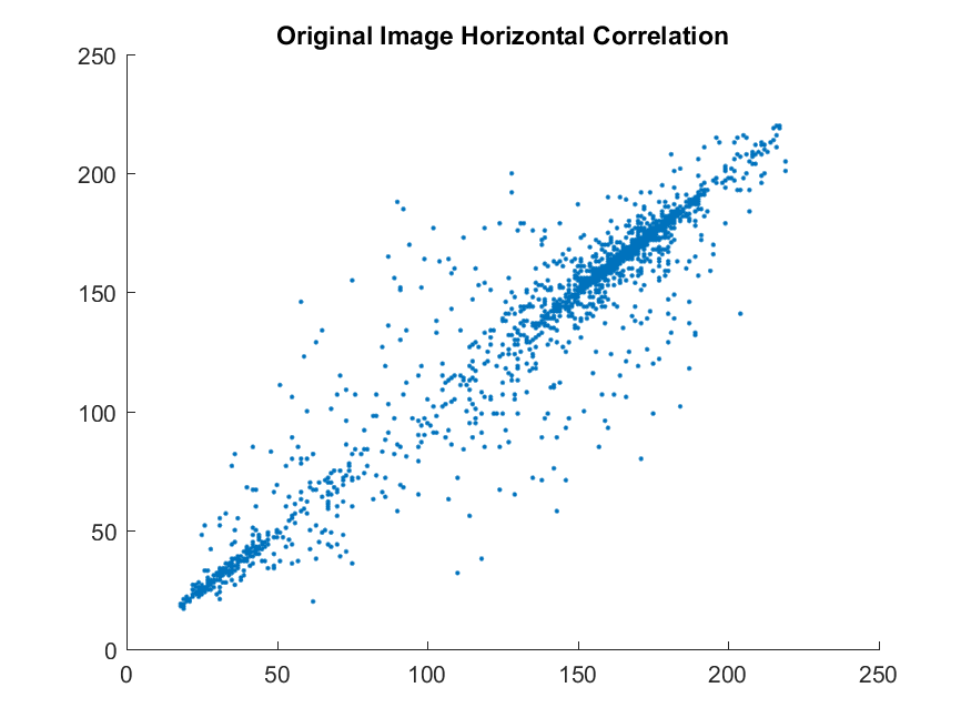
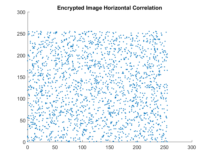
In image processing, correlation is used for matching templates (template matching resource). The idea is to check if the encrypted image is similar to a given template, the template being an adjacent pixel. How? Well, correlation between adjacent pixels can be used to detect patterns.
Usually, academic literature provides results of pixel correlation using either tables or scatter plots (sometimes they give both which makes no sense). I, personally, prefer tables because they reduce the number of pages which can be a big problem while writing academic papers. The scatterplots look like this:
 |
|---|
| Horizontal correlation for the plain image - High Correlation |
 |
|---|
| Horizontal correlation for the encrypted image - Low Correlation |
These plots are created by selecting around 2000 pairs of horizontally adjacent pixels in the original and encrypted images. The correlation between the pixels can be directly calculated using the inbuilt functions in the tool you are using (most probably Matlab or OpenCV). The values are between -1 and 1. In the case of encryption, we usually ignore the sign. If the correlation is close to 0, it means the two images are not correlated and the encryption has been successful.
2. Number of Pixel Change Ratio (NPCR) and Unified Average Change Intensity (UACI)
Another word of caution: NPCR and UACI are famous for being unreliable. The current cryptography algorithms are strong enough to last a few more decades without breaking a sweat. But there is an influx of cryptography techniques which are poorly constructed and evaluated using unsuitable metrics. Calculating NPCR and UACI are common among them. If you are reading a paper where a key is generated using some kind of chaotic function, you should start looking somewhere else. These methods have long been proven as insecure. Here’s an example. Such papers regularly crop up in cryptography-adjacent journals due to the pressure to publish in academia. These papers are usually written by people who are not savvy with crypto techniques. For a good encryption technique, there needs to be a suitable proof in the paper which shows that the encryption is secure along with it’s time and space complexities.
NPCR and UACI are the metrics that have inspired this post. Most of the students who came to me had a problem understanding these. To understand these metrics, the reader should know about differential attacks. Although an in-depth knowledge is not required, I would recommend the reader to go through this Wikipedia article.
NPCR and UACI are used to check the resistance of the encryption technique to differential attacks. Differential attacks tell us how changes in the plain text affect the cipher text. Thus, we can track if a minor change in the original pixel value propagates or gets amplified in the encrypted image. To calculate this metric, we need two images.
- Original encrypted image
- Encrypted image generated after toggling 1 LSB in a random pixel of the original plain image.
If the two encrypted images are represented by $C_1$ and $C_2$. Then, the NPCR and UACI are calculated using the following equations
\[D(i, j) = \begin{cases} 0, & \text {if } C_1(i, j) = C_2(i, j) \\ 1, & \text {if } C_1(i, j) \neq C_2(i, j) \end{cases}\]\[NPCR = \sum_{i, j} \frac {D(i, j)}{N}\]
\[UACI = \sum_{i, j} \frac {C_1(i, j) - C_2(i, j)}{L \times N}\]
where $N$ is the number of pixels in the encrypted image and $L$ is the max intensity level possible for the image. So, $L$ would be 2 for a binary image, 255 for a 8-bit image, and so on.
According to the literature, a value approximately equal to 1 for NPCR and around 0.33 for UACI imply the techniques are secure. These values have been set empirically and there is no specific proof and hence, these metrics are considered unreliable.
But people use them anyways 🤷♂️.
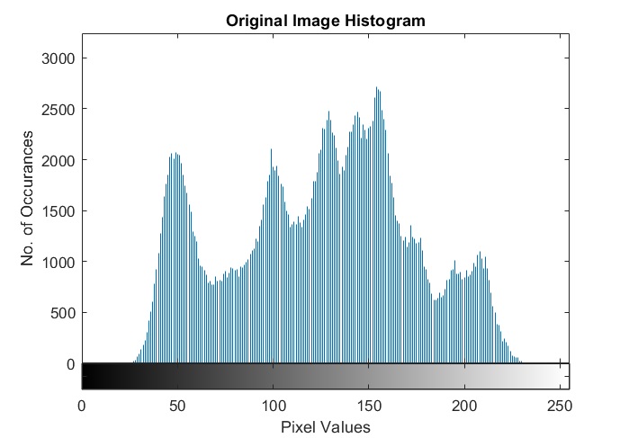
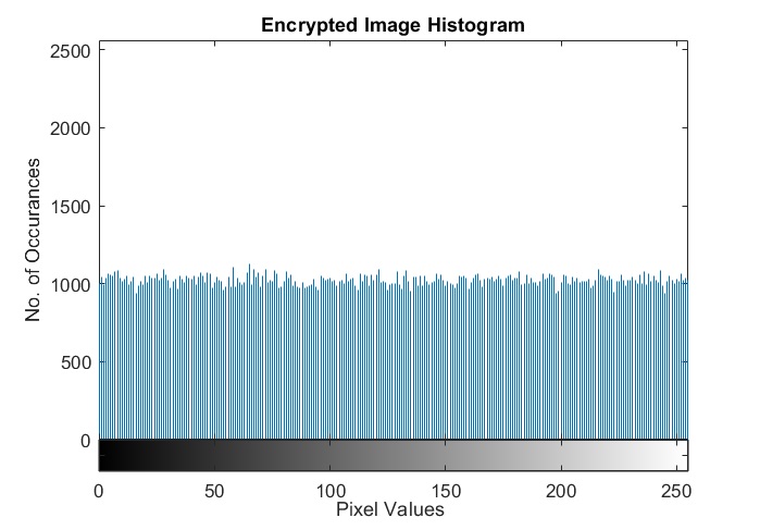
3. Histogram analysis
The histogram of an encrypted image should be flat. This signifies that all the pixel values are equiprobable. Here is an example of histograms of a normal image and an encrypted image. In this case, I have taken Lena as the plain image and encrypted it with the one time pad scheme.
 |  |
|---|---|
| Histogram of plain image | Histogram of encrypted image |
4. Robustness
This metric indicates the resistance of the encryption technique to noise and attacks like cropping, shearing and rotating the encrypted image. This metric is usually shown by cropping a part of the encrypted image and the showing the decrypted image as given below. The idea here is to determine how much of the original image can be recovered if a malicious entity performs operations like cropping on the encrypted image. As seen in the figure below, the decrypted image is reasonably clear even after 25% of the encrypted pixels have been reset.
 | 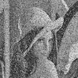 |
|---|---|
| Encrypted Image with 25% of the pixels removed | Decryption of the incomplete image |
5. Key space analysis
Key space analysis basically tells us the number of possible keys for a given encryption algorithm. An important factor to consider here is that this metric is an analysis and the researcher must give a proof of the length of the key space for the given cipher. A larger key space would make the cipher more difficult to break.